Custom derived quantities

When you fit an SED with galapy-fit, the sampler explores the posterior of the free model parameters (ages, star-formation parameters, ISM parameters, …). On their own those numbers are rarely what you want to report. What you usually report are derived quantities; i.e. physical numbers computed from the model at each posterior sample: a stellar mass, a star-formation rate, a dust temperature, a model SED.

galapy computes a set of these for you automatically and stores their full posterior (one value per sample) inside the Results object. This guide shows you how to

1. choose which built-in quantities are stored when you run a fit,

2. add your own quantities to an existing Results object, and

3. summarise any of them (mean, median, credible intervals).

It builds up in four levels — feel free to stop at the one that covers your use case. The cookbook at the end collects ready-to-paste recipes.

The built-in quantities

Every Results object stores the posterior of these nine quantities by default:

key	quantity	units	shape
SED	spectral energy distribution	flux, mJy	array
Mstar	stellar mass	\(M_\odot\)	scalar
Mdust	dust mass	\(M_\odot\)	scalar
Mgas	gas mass	\(M_\odot\)	scalar
Zstar	stellar metallicity	absolute (metal mass fraction)	scalar
Zgas	gas metallicity	absolute (metal mass fraction)	scalar
SFR	star-formation rate	\(M_\odot\) / yr	scalar
TMC	molecular-cloud temperature	K	scalar
TDD	diffuse-dust temperature	K	scalar

Each is exposed as an attribute holding the posterior: a (Nsamples,) array for the scalar quantities and a (Nsamples, Nwavelength) array for the SED.

from galapy.sampling.Results import load_results

# load a results file written by galapy-fit (HDF5 or pickle); the format is
# inferred from the extension
res = load_results( 'data/sampling_4D+noise_dynesty_results_light.galapy.hdf5' )

res.Mstar.shape   # -> (Nsamples,)
res.SED.shape     # -> (Nsamples, Nwl)
res.get_stored_quantities()   # everything currently stored on this object

Read from file data/sampling_4D+noise_dynesty_results_light.galapy.hdf5
Now processing the sampling results, this might require some time ...
... done in 35.92068648338318 seconds.

['_mod',
 '_han',
 'Ndof',
 '_obs',
 '_noise',
 'sampler',
 'ndim',
 'logz',
 'logzerr',
 'size',
 'params',
 'logl',
 'samples',
 'weights',
 'wnot0',
 '_derived',
 'SED',
 'Mstar',
 'Mdust',
 'Mgas',
 'Zstar',
 'Zgas',
 'SFR',
 'TMC',
 'TDD']

Level 1 — choosing which built-ins to store (no code)

Computing and storing every quantity for every posterior sample takes time and disk space (the SED in particular is a full array per sample). If you only care about a few numbers, tell galapy-fit to store just those, through the store_quantities hyperparameter in your parameter file:

# parameter file (galapy-genparams)
store_quantities = ['Mstar', 'SFR', 'Mdust']

• None (the default) stores all nine quantities.

• A shorter list makes the output file smaller and post-processing faster.

• 'SED' is always stored, whether or not you list it — listing it just prints a harmless warning and is ignored. (The SED is needed internally to validate each sample, so you always get it for free.)

That is all most users ever need. The remaining levels are for when you want a quantity that is not in the built-in list.

Level 2 — adding one custom quantity

Anything you can compute from a fully-configured galapy model, you can store as a derived quantity, after the run, with Results.add_property.

You pass a function that takes one argument, the model, with the parameters of the current sample already set, and returns the value you want for that sample:

# bolometric-ish luminosity: integrate the model SED
res.add_property( lambda model : model.get_SED().sum(), name = 'Lsed' )

res.Lsed.shape   # -> (Nsamples,)  one value per posterior sample

(13093,)

add_property evaluates your function on every posterior sample exactly the way the built-ins are evaluated, stores the result as a new attribute (res.Lsed here), and returns the list of names it added:

res.add_property( lambda model : model.age, name = 'age' )
# -> ['age']

What can the model give you? Anything the model exposes, for example:

model.age                       # galaxy age [yr]
model.sfh.Mstar( model.age )    # stellar mass at that age
model.sfh( model.age )          # SFR at that age
model.ism.mc.T                  # molecular-cloud temperature
model.get_SED()                 # the model SED [mJy]
model.get_emission()            # rest-frame luminosity [Lsun]

If you omit name for a single function, it is auto-named custom0, custom1, … — handy for quick exploration, but pass an explicit name for anything you intend to keep.

⚠️ The operation of adding a new property to the list can take up to several 10s of seconds. This is a consequence of the necessity to re-build the model for each sample in the parameter space. Since this additional cost is payed every time you call add_property, in the case you need to store more than 1 additional quantity, it is desirable to list all of them in a single call of add_property, as explained in the following section.

Level 3 — several quantities at once, and summarising them

To add more than one quantity in a single pass over the posterior, hand add_property a dictionary of { name : function }. The posterior is walked once and all the functions are evaluated per sample. Way cheaper than calling ``add_property`` repeatedly:

res.add_property( {
    'Lsed'   : lambda model : model.get_SED().sum(),
    'fdust'   : lambda model : model.sfh.Mdust( model.age ) / model.sfh.Mstar( model.age ),
} )
# -> ['Lsed', 'fdust']

['Lsed', 'fdust']

Once stored, a custom quantity behaves exactly like a built-in: every summary helper accepts its name.

res.get_mean( 'fdust' )                          # posterior weighted mean

np.float64(0.03117078069462907)

res.get_median( 'fdust' )                         # posterior median

np.float64(0.03183249464890653)

res.get_quantile( 'fdust', quantile = 0.84 )      # any weighted quantile

np.float64(0.0326207884865276)

res.get_std( 'fdust' )                            # weighted standard deviation

np.float64(0.0017871797022055297)

res.get_bestfit( 'fdust' )                        # value at the max-likelihood sample

np.float64(0.032246973058956345)

res.get_credible_interval( 'fdust', percent = 0.68 )   # central 68% interval

(np.float64(0.0014986467092172572), np.float64(0.0007044928481782092))

These helpers are posterior-weighted (they use the sampling weights) and they automatically exclude invalid samples (see the sentinel note below), so you do not have to filter anything by hand.

Level 4 — array-valued quantities, and a numerical pitfall

A derived quantity can be an array, not just a scalar — the SED is the built-in example. The classic user case is the average attenuation curve as a function of wavelength.

It is tempting to store the attenuation in magnitudes via the model’s get_avgAtt(). Do not — and this is the single most common trap, so it gets its own box:

⚠️ Average in linear space, not in magnitudes / logs. Magnitude attenuation is -2.5 * log10( attenuated / unattenuated ). When a sample attenuates a band to (near) zero flux that is +inf; round-off can even make it nan. Those non-finite values are correct per sample, but they poison any posterior mean. Store the linear quantity and convert at the very end. For attenuation, galapy already keeps the linear average attenuation factor (in [0, 1]) on the model as model.Aavg after every parameter update:

res.add_property( lambda model : model.Aavg, name = 'Aavg' )

res.Aavg.shape                  # -> (Nsamples, Nwl), finite by construction
mean_Aavg = res.get_mean( 'Aavg' )      # safe: linear, finite

# convert the *summary* to magnitudes only at the end, if you want them:
import numpy as np
mean_att_mag = -2.5 * np.log10( mean_Aavg )

The same principle applies to any quantity you would normally view in log space (luminosities spanning orders of magnitudes, metallicities, …): store it linear, average, then take the log of the summary.

Saving the newly computed derived properties

Custom quantities are first-class: they are serialised together with the built-ins, so you only pay the per-sample evaluation cost once. After adding properties you can re-save the Results object and reload it later.

The lowest-friction option is to pickle the whole object:

import pickle
res.add_property( lambda model : model.Aavg, name = 'Aavg' )

with open( 'myfit_with_Aavg.pickle', 'wb' ) as f :
    pickle.dump( res, f )

from galapy.sampling.Results import load_results
later = load_results( 'myfit_with_Aavg.pickle' )   # format inferred from extension
later.get_mean( 'Aavg' )        # the custom quantity is right there

To re-save as HDF5 instead (portable, the format galapy-fit uses), dump the object to a dictionary and write it with the galapy IO helper:

import galapy
from galapy.io.hdf5 import write_to_hdf5

write_to_hdf5(
    'myfit_with_Aavg.galapy.hdf5',
    metadata = dict( storage_method = 'hard',
                     galapy_version = galapy.__version__ ),
    hard     = True,
    results  = res.dump(),
)
later = load_results( 'myfit_with_Aavg.galapy.hdf5' )

(Under the hood the in-memory round-trip is Results.load( res.dump() ): dump() returns a plain dictionary and Results.load() rebuilds the object from it — load_results is just the file-level wrapper around that.)

ℹ️ Invalid samples are flagged, not dropped. If a sample’s parameters are unphysical (e.g. its SED is non-finite), every derived quantity for that sample is stored as -inf rather than silently skipped, so all the per-sample arrays keep the same length and stay aligned with the chain. The summary helpers exclude these sentinels automatically; if you slice the raw arrays yourself, mask them with numpy.isfinite first.

Cookbook

Short, paste-ready recipes. Each assumes a loaded Results object res.

Specific star-formation rate (sSFR):

res.add_property(
    lambda model : model.sfh( model.age ) - model.sfh.Mstar( model.age ),
    name = 'sSFR' )

Dust-to-stellar mass ratio:

res.add_property(
    lambda model : model.sfh.Mdust( model.age ) - model.sfh.Mstar( model.age ),
    name = 'fdust' )

Monochromatic luminosity at a chosen rest-frame wavelength (e.g. 1500 Å):

import numpy as np
def L1500 ( model ) :
    wl = model.wl()                       # rest-frame wavelength grid [Angstrom]
    return np.interp( 1500., wl, model.get_emission() )
res.add_property( L1500, name = 'L1500' )

A rest-frame colour from the model SED (flux ratio in two windows):

import numpy as np
def colour ( model ) :
    wl, sed = model.wl(), model.get_SED()
    blue = sed[ ( wl > 4000. ) & ( wl < 5000. ) ].mean()
    red  = sed[ ( wl > 6000. ) & ( wl < 7000. ) ].mean()
    return -2.5 * np.log10( blue / red )      # scalar -> magnitudes is fine here
res.add_property( colour, name = 'blue_red' )

(Here the per-sample value is finite, so magnitudes are safe — contrast with the average-attenuation case, where it is the averaging across samples that breaks.)

Linear average attenuation curve (then convert the summary):

res.add_property( lambda model : model.Aavg, name = 'Aavg' )
att_mag_median = -2.5 * np.log10( res.get_median( 'Aavg' ) )

Several quantities in one pass:

res.add_property( {
    'sSFR'  : lambda model : model.sfh( model.age ) / model.sfh.Mstar( model.age ),
    'fdust' : lambda model : model.sfh.Mdust( model.age ) / model.sfh.Mstar( model.age ),
    'Lsed'  : lambda model : model.get_SED().sum(),
} )

Plotting

The posteriors of derived properties added via add_property can be plotted through the corner_derived helper function along with the default derived properties:

from galapy.analysis.plot import corner_derived

fig, axes = corner_derived(
    res, which_keys = [
        'SFR', 'TMC', 'TDD', # <-- default
        'fdust', 'Lsed'      # <-- custom
    ],
    getdist_settings={
        'contours' : [0.68, 0.95],
        'smooth_scale_2D' : 0.5,
        'fine_bins': 1024,
        'fine_bins_2D': 1024,
    },
)

Removed no burn in

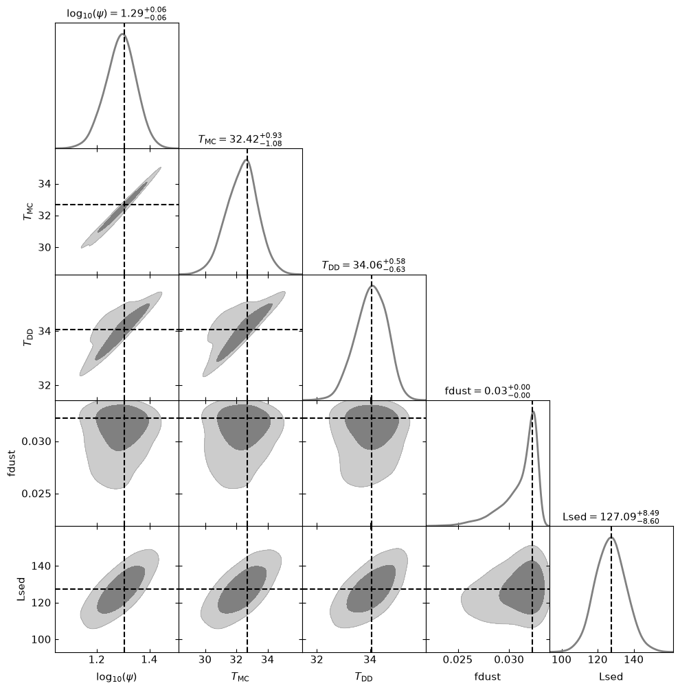
Since a user-defined property does not have built-in metadata, corner_derived falls back to showing the quantity’s name as the axis label (rendered as, e.g., Lsed or fdust, above). Built-in quantities, by contrast, get a nice LaTeX symbol (\(\psi\), \(T_\mathrm{MC}\), \(T_\mathrm{DD}\) above).

Label and log-axis choices for the derived quantities live entirely on the analysis-side: they are not stored. You can supply them at plotting time through keyword arguments:

• labels: a {key: latex} dictionary giving a LaTeX symbol for a quantity (raw LaTeX, no surrounding $ are required);

• log_scale: a list of keys to draw on a log10 axis.

For example, having added Lsed and fdust:

fig, axes = corner_derived(
    res, which_keys = [
        'SFR', 'TMC', 'TDD', # <-- default
        'fdust', 'Lsed'      # <-- custom
    ],
    labels = {
        'Lsed' : 'L_\mathrm{SED}',  # proper symbol instead of Lsed
        'fdust' : 'f_\mathrm{dust}' # proper symbol instead of fdust
    },
    log_scale = ['SFR', 'fdust'],    # fdust on log-axis too
    getdist_settings={
        'contours' : [0.68, 0.95],
        'smooth_scale_2D' : 0.5,
        'fine_bins': 1024,
        'fine_bins_2D': 1024,
    },
)

Removed no burn in

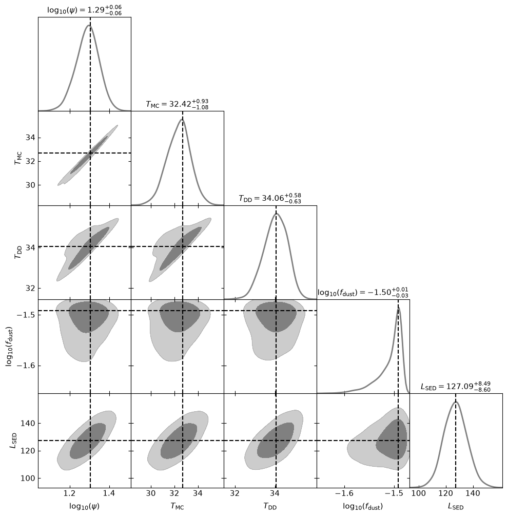
The labels mapping also overrides the default label of a built-in quantity if you list it, and the \log_{10}(...) wrapping is applied automatically on top of a label whenever the corresponding key also appears in the log_scale list.

Since these are purely cosmetics the same Results object can be re-plotted with different labels without changing anything stored in it.

Recap

• Storing built-ins: set store_quantities in the parameter file; SED is always kept.

• Adding your own: res.add_property( f, name = ... ), where f(model) returns the per-sample value; pass a dict to add several at once.

• Summarising: get_mean, get_median, get_quantile, get_std, get_bestfit, get_credible_interval — all accept custom names and are posterior-weighted.

• Two rules that save you: return the same shape for every sample, and average linear quantities in linear space (convert to log/mag only at the end).